Parallel Group- or Cluster-Randomized Trials (GRTs)

In a parallel group-randomized trial (GRT), also called a parallel cluster-randomized trial, groups or clusters are randomized to study conditions, and observations are taken on the members of those groups with no cross-over of groups or clusters to a different condition or study arm during the trial (Campbell and Walters, 2014; Donner and Klar, 2000; Eldridge and Kerry, 2012; Hayes and Moulton, 2017; Murray, 1998). This design is common in public health, where the units of assignment may be schools, worksites, clinics, or whole communities, and the units of observation are the students, employees, patients, or residents within those groups. It is common in animal research, where the units of assignment may be litters of mice or rats and the units of observation are individual animals. It is also common in clinical research, where the units of assignment may be patients and the units of observation are individual teeth or eyes. Special methods are needed for analysis and sample size estimation for these studies, as detailed below and in the parallel GRT sample size calculator.

Features and Uses

Public Health and Medicine

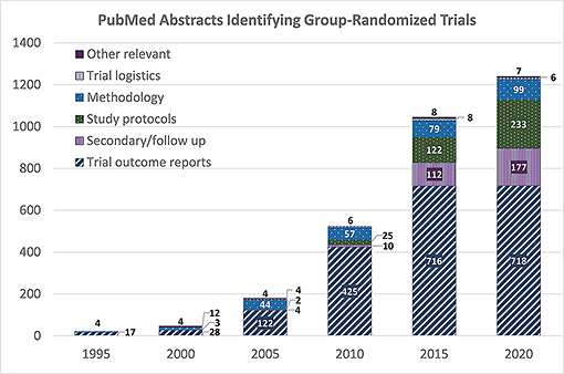
The GRT design is increasingly common in public health and medicine, and the literature on the design, analysis, and use of GRTs has grown rapidly over the last 25 years. The accompanying figure demonstrates this growth, showing that the number of PubMed abstracts that identify GRTs for human studies more than doubled every 5 years from 1995 through 2015, with continued but less dramatic growth through 2020.

Animal Research

Parallel GRTs are common in animal research, where the units of assignment may be litters of mice or rats, or other collections of animals. The design and analytic issues are the same, whether the study involves human or animals, and whether the research is applied or basic.

Nested or Hierarchical Design

Parallel GRTs have a nested or hierarchical design: the groups randomized to each study condition are nested within those study conditions so that each group appears in only one study condition.

The members are nested within those groups so that each member appears in only one group. In cohort GRTs, members are observed repeatedly so that measurements are nested within members; in cross-sectional GRTs, different members are observed in each group at each measurement occasion. In each case, the units of observation are nested within the units of assignment, which are nested within the study conditions.

Appropriate Use

Parallel GRTs can be employed in a wide variety of settings and populations to address a wide variety of research questions. They are the best comparative design available when the investigator wants to evaluate an intervention that:

  • operates at a group level,
  • manipulates the social or physical environment, or
  • cannot be delivered to individual participants without substantial risk of contamination.

Potential for Confounding

Parallel GRTs often involve a limited number of groups randomized to each study condition. A recent review found that the median number of groups randomized to each study condition in GRTs related to cancer was 25, though many were much smaller (Murray et al., 2018). When the number of groups available for randomization is limited, there is a greater risk that potentially confounding variables will be unevenly distributed among the study conditions, and this can threaten the internal validity of the trial. As a result, when the number of groups to be randomized to each study condition is limited, a priori matching and a priori stratification are widely recommended to help ensure balance across the study conditions on potential confounders (Campbell and Walters, 2014; Donner and Klar, 2000; Hayes and Moulton, 2017; Murray, 1998

) More recently, constrained randomization is recommended as another option for parallel GRTs (Li et al., 2016; Li et al., 2017b).

Intraclass Correlation

The more challenging feature of parallel GRTs is that members of the same group usually share some physical, geographic, social, or other connection. Those connections create the expectation for a positive intraclass correlation (ICC) among observations taken on members of the same group, as members of the same group tend to be more like one another than to members of other groups. The ICC is simply the average bivariate correlation on the outcome among members of the same group or cluster.

Positive ICC reduces the variation among the members of the same group but increases the variation among the groups. As such, the variance of any group-level statistic will be larger in a parallel GRT than in a randomized clinical trial (RCT). Complicating matters further, the degrees of freedom (df) available to estimate the ICC or the group-level component of variance will be based on the number of groups, and so are often limited. Any analysis that ignores the extra variation (or positive ICC) or the limited df will have a type I error rate that is inflated, often badly (Campbell and Walters, 2014; Donner and Klar, 2000; Eldridge and Kerry, 2012; Hayes and Moulton, 2017; Murray, 1998).

Solutions

The recommended solution to these challenges is to employ a priori matching, a priori stratification, or constrained randomization to balance potential confounders, to reflect the hierarchical structure of the design in the analytic plan; and to estimate the sample size for the GRT based on realistic and data-based estimates of the ICC and the other parameters indicated by the analytic plan. Extra variation and limited df always reduce power, so it is essential to consider these factors while the study is being planned, and particularly as part of the estimation of sample size.

The sections below provide additional resources for investigators considering a parallel group- or cluster-randomized trial.


FAQs

Use a parallel GRT if you have an intervention that operates at a group level, manipulates the social or physical environment, or simply cannot be delivered to individuals without serious risk of contamination. If you can deliver your intervention to individuals without risk of contamination and can avoid interaction among participants post-randomization, it is more efficient and easier to use a traditional RCT.

A pragmatic trial is one that helps users choose between options for care. These trials are usually done in the real world, under less well-controlled conditions than more traditional clinical trials. Pragmatic trials can use a traditional RCT design, or they can use a parallel GRT design. Stepped wedge group-randomized trials (SW-GRTs) are also used in pragmatic trials. Of 21 pragmatic trials supported by the Health Care Systems Research Collaboratory at the NIH, two are RCTs, 10 are GRTs, four are IRGTs, and five are SWGRTs.

There are five published textbooks on the design and analysis of group- or cluster-randomized trials (Campbell and Walters, 2014; Donner and Klar, 2000; Eldridge and Kerry, 2012; Hayes and Moulton, 2017; Murray, 1998). A recent textbook is devoted to power and sample size calculation for multilevel designs, including parallel GRTs, IRGTs, and stepped wedge group-randomized trials (Moerbeek and Teerenstra, 2016).

Yes. Sometimes investigators randomize months or weeks within clinics to study conditions. As an example, consider a study in which over the course of a year, six months are spent delivering the intervention condition and six months are spent delivering the control condition, with the order randomized within each clinic. The unit of assignment in this case is the time block within the clinic, rather than the clinic itself. Patients receive the intervention or control condition appropriate to the time block when they come to the clinic. While these groups are not structural groups like whole clinics, they are still groups, and this is still a parallel group- or cluster-randomized trial with the time block as the group. The key number in this case for power or sample size calculations is the number of time blocks, not the number of clinics. In this example, the clinic is crossed with study conditions as there are both interventions and control participants in each clinic; the clinic can be included in the analysis as a fixed effect stratification factor and that may improve power. 

It is important to distinguish between changing study conditions or study arms and changing groups or clusters. In a parallel GRT or IRGT, it is important to ensure that each participant remains in the study condition to which they were randomized. Those assigned to the intervention condition should not move to the control condition, and vice versa. Sometimes that is unavoidable, but it should be uncommon. If it does happen, standard practice is to analyze as randomized, under the intention-to-treat principle.

The other possibility is that a participant in a GRT or IRGT would change groups or clusters even as they stay in the same study condition or study arm. In a school-based trial, a participant from one intervention school might move to another intervention school. Or in an IRGT, a participant who usually went to the Tuesday night class might sometimes go to the Saturday morning class. Recent studies have shown that failure to account for changing group membership can result in an inflated type I error rate (Andridge et al., 2014). Several authors provide methods for analyzing data to account for such changes (Candlish et al., 2018; Luo et al., 2015; Roberts and Walwyn, 2013; Sterba, 2017).

Standard sources assume that each group or cluster has the same number of observations, but that is almost never true in practice. So long as the coefficient of variation (CV) of group size is less than 0.23, such variation can be ignored (Eldridge et al., 2006). But as the variation grows more marked, analysts risk an inflated type I error rate if they ignore it (Johnson et al., 2015).

In addition, power falls as the variation in group or cluster size increases, so that it needs to be addressed in the sample size calculations. There are a number of publications on this issue for GRTs (Candel and van Breukelen, 2010; Candel and van Breukelen, 2016; Hemming et al., 2020; Lauer et al., 2015; Liu et al., 2021; Moerbeek and Teerenstra, 2016; van Breukelen et al., 2007; Wang et al., 2020; Xu et al., 2019; You et al., 2011). There are also a few publications on this issue for IRGTs (Candel and van Breukelen, 2009; Moerbeek and Teerenstra, 2016).

We have known for some time that the magnitude of the ICC is inversely related to the level of aggregation (Donner, 1982). The smaller the level of aggregation, the larger the ICC. Spouse pairs and family units are small clusters, so their ICCs are often large. Moving to larger aggregates, like worksites or schools, the ICCs are usually smaller. Moving to even larger aggregates, like communities, the ICCs are usually even smaller. However, the ICC is not the only factor that determines sample size in a GRT. The variance inflation factor is defined as (1+(m-1)ICC) where m is the average number of observations in the groups randomized in the study. In a spouse pair, m=2, so that the formula is reduced to 1+ICC, and the VIF will be less than 2. If a school study, the ICC may be much smaller, e.g., 0.05, but the number of observations may be much larger, e.g., 400, and the VIF=1+(400-1)0.05=20.95, which will have a much more deleterious effect on the power of the study. It is important to account for the ICC, but also the average number of observations expected in each group randomized to the study conditions, as well as the number of groups randomized, as that dictates the df available for the test of the intervention effect. These issues are discussed in Part 4 of the Pragmatic and Group-Randomized Trials in Public Health and Medicine Course.

It is true that this approach will improve the fidelity of implementation. But the problem is that this approach completely confounds the instructor/facilitator with the study condition: everyone who gets the intervention gets exposed to that instructor/facilitator. In that situation, it is impossible to separate the effect of the intervention from the effect of the instructor/facilitator. It is possible that a charismatic instructor/facilitator could generate beneficial effects on the outcome of interest, even if the intervention itself is completely ineffective, and the investigator would not be able to distinguish those two effects. It is better to use an IRGT design in which multiple instructors/facilitators are used in the intervention condition so that variability due to instructors/facilitators can be separated from variability due to the intervention. 

In a parallel GRT, the groups are the units of assignment and are nested within study conditions, with different groups in each condition. In an IRGT, the groups are created in the intervention condition to facilitate delivery of the intervention; those groups may be defined by their instructor or facilitator, surgeon, therapist, or other interventionist, or they may be virtual groups. So long as the groups are nested within study conditions, they must be included in the analysis as levels of a random effect; ignoring them, or including them as levels of a fixed effect, will result in an inflated type 1 error rate. That is true for GRTs (Campbell and Walters, 2014; Donner and Klar, 2000; Eldridge and Kerry, 2012; Hayes and Moulton, 2017; Murray, 1998) and for IRGTs (Baldwin et al., 2011; Bauer et al., 2008; Candlish et al., 2018; Kahan and Morris, 2013; Lee and Thompson, 2005a; Lee and Thompson, 2005b; Pals et al., 2008; Pals et al., 2011; Roberts and Roberts, 2005; Roberts and Walwyn, 2013). This is because nested factors must be modeled as random effects (

Zucker, 1990

). 

This explanation also offers a potential solution – if the investigator can avoid nesting groups within study conditions, the requirement to model those groups as levels of a random effect disappears. The alternative to nesting is crossing, so if it is possible to cross the levels of the grouping factor with study conditions, then the grouping factor becomes a stratification factor and the investigator is free to model the grouping factor as a random effect, as a fixed effect, or to ignore the grouping factor in the analysis. –

For example, if schools are randomized to study conditions, the study is a GRT. But if students within schools are randomized to study conditions, the schools will be crossed with study conditions and we have a stratified RCT; the investigator can model the schools as a random effect, as a fixed effect, or ignore it in the analysis. As another example, if the therapists used to deliver the intervention in an IRGT also deliver an alternative intervention in the control condition, the therapists will be crossed with study condition and the investigator can model therapist as a random effect, as a fixed effect, or ignore therapist in the analysis. In either example, the choice between modeling the grouping factor as random, as fixed, or ignoring it will depend on factors like power and generalizability.

The best estimate for the ICC will reflect the circumstances for the trial being planned. That estimate will be from the same target population, so that it reflects the appropriate groups or clusters (e.g., schools vs. clinics vs. worksites vs. communities); age groups (e.g., youth vs. young adults vs. seniors); ethnic, racial, and gender diversity; and other characteristics of the target population. That estimate will derive from data collected for the same outcome using the same measurement methods to be used for the primary outcome in the trial being planned. For example, if planning a trial to improve servings of fruits and vegetables in inner-city third graders, it would be important to get an ICC estimate for servings of fruits and vegetables, measured in the same way as servings would be measured in the trial being planned, from third-graders in inner-city schools like the schools that would be recruited for the trial being planned.

Regression adjustment for covariates often improves power in a GRT or IRGT by reducing the residual error variance or the ICC (Murray and Blitstein, 2003). At the same time, it is important to remember that regression adjustment for covariates can reduce power in a GRT or IRGT by increasing the ICC (Murray, 1998). As such, it is important to choose covariates carefully. The best covariates will be related to the outcome and unevenly distributed between the study conditions or among the groups or clusters randomized to the study conditions.

A priori matching can improve power in a GRT, but it can also reduce power, so investigators need to be thoughtful about a priori matching in their design and analysis. A priori matching reduces the df for the test of the intervention effect by half, and if the correlation between the matching factor and the outcome is not large enough to overcome the loss of df, power will be reduced in the matched analysis compared to the unmatched analysis.

A priori matching is often used to balance potential confounders, and it is then up to the investigator to decide whether to reflect that a priori matching in the analysis. It is not required, because the type 1 error rate is unaffected when the matching or stratification factor is ignored in the analysis of intervention effects (Diehr et al., 1995; Proschan, 1996). However, Donner et al., 2007 have warned against ignoring matching in analyses that do not involve intervention effects, e.g., in an analysis to examine the association between a risk factor and an outcome. Ignoring matching in the analysis in this situation can lead to an inflated type 1 error rate when the correlation between the matching factor and either the outcome or the risk factor is at least modest (>0.2) and the number of members per group is not large (<100). Stratification with strata of size four avoids this problem and improves efficiency almost as much as matching. For this reason, stratification with strata of size four is a prudent strategy for balancing potential confounders across study conditions or study arms.

A priori stratification can also improve power in a GRT, but the situation is more complicated, because it depends on how the stratification is reflected in the analysis. As with a priori matching, a priori stratification can be used to balance potential confounders, and it is then up to the investigator to decide whether and how to reflect that a priori stratification in the analysis.

If the primary interest is to balance on potential confounders, the stratification factor could be included in the analysis as a covariate, but without creating interactions with study condition or other factors. To the extent that the stratification factor is related to the outcome, there is likely to be benefit to power, because the gain from the regression adjustment is likely to outweigh any reduction due to lost df.

If the primary interest is differential intervention effects, the stratification factor is included in the analysis as a main effect, but additional interaction terms are required, both for fixed and random effects. The number and nature of the additional fixed and random effects will depend on the design and analytic plan (Murray, 1998; Murray, 2001). Inclusion of the correct fixed and random effects is essential to a valid analysis, so investigators are strongly encouraged to work with a methodologist familiar with stratified designs to ensure that the analysis is structured correctly. Regarding power, detection of differential intervention effects will always require a larger study than detection of uniform intervention effects.

Constrained randomization is an alternative to a priori matching or stratification (Li et al., 2016; Li et al., 2017b). It can be used to balance across a larger number of covariates than is typically possible with matching or stratification, usually improves power, and can be used either with model-based or permutation-based tests.

Some have suggested that 4 groups or clusters per study condition should be considered as an absolute minimum (Hayes and Moulton, 2017). Investigators should be cautious about such rules of thumb because it is quite possible that 4 groups or clusters per study condition would result in a badly underpowered trial. ICCs in public health and medicine often fall in the range of 0.01–0.05, and if the ICC does fall in that range, 8–12 groups or clusters will often be needed in each study condition. The best advice is to estimate sample size requirements for the trial under consideration, using the best parameter estimates available.

There is no general answer to this question. Instead, investigators should estimate sample size requirements for the trial under consideration, using the best parameter estimates available. At the same time, it is fair to say that increasing the number of groups or clusters per condition will more effectively increase power than will increasing the number of members per group or cluster.

No. When a priori matching or stratification is used for balance, the matching or stratification factor may be included in the analysis of intervention effects, but that is not required, and it may be inefficient to do so. It is not required because the type 1 error rate is unaffected when the matching or stratification factor is ignored in the analysis of intervention effects (Diehr et al., 1995; Proschan, 1996). Both procedures reduce the df available for the test of the intervention effect, and if the number of df is limited, the unmatched or unstratified analysis may be more powerful than the matched or stratified analysis. In that circumstance, it is to the investigator’s advantage to match or stratify in the design to achieve balance on potential confounders, but to ignore the matching or stratification in the analysis to improve power or reduce sample size (Diehr et al., 1995). The choice of whether to include the matching or stratification factor in the analysis should be made a priori based on sample size calculations comparing the matched or stratified analysis to the unmatched or unstratified analysis.

The choice between a priori matching and a priori stratification for balance should be guided by whether the investigator anticipates doing analyses that do not involve intervention effects. Donner et al., 2007 have warned against ignoring matching in analyses that do not involve intervention effects, e.g., in an analysis to examine the association between a risk factor and an outcome. Ignoring matching in the analysis in this situation can lead to an inflated type 1 error rate when the correlation between the matching factor and either the outcome or the risk factor is at least modest (>0.2) and the number of members per group is not large (<100). Stratification with strata of size four avoids this problem and improves efficiency almost as much as matching. For this reason, stratification with strata of size four is a prudent strategy for balancing potential confounders across study conditions because it is almost as efficient as matching, and it does not limit the range of analyses that can be applied to the data.

No. In public health and medicine, ICCs in group- or cluster-randomized trials are often small, usually ranging from 0.01–0.05 (Moerbeek and Teerenstra, 2016). While it is tempting to ignore such small correlations, doing so risks an inflated type I error rate, and the risk is substantial both in parallel GRTs (Campbell and Walters, 2014; Donner and Klar, 2000; Eldridge and Kerry, 2012; Hayes and Moulton, 2017; Murray, 1998) and in IRGTs (Baldwin et al., 2011; Bauer et al., 2008; Candlish et al., 2018; Kahan and Morris, 2013; Lee and Thompson, 2005b; Lee and Thompson, 2005a; Pals et al., 2011; Pals et al., 2008; Roberts and Roberts, 2005; Roberts and Walwyn, 2013). The prudent course is to reflect all nested factors as random effects and to plan the study to have sufficient power given a proper analysis.

No. That is another tempting strategy that can risk an inflated type I error rate. The standard error for the variance component is not well estimated when the value is close to zero, and if the df are limited, the power will be limited. As such, it is likely that the result will suggest that the ICC or variance component is negligible, when ignoring it will inflate the type I error rate. The prudent course is to reflect all nested factors as random effects and to plan the study to have sufficient power given a proper analysis.

There are three common analytic models used for pretest-posttest parallel GRTs. (Murray, 1998).

First, one could analyze the posttest data, ignoring the pretest data altogether.

Second, one could analyze the posttest data with regression adjustment for covariates measured at baseline, including adjustment for the baseline measure of the outcome, as is common in a cohort design.

Because the second approach includes regression adjustment for covariates, it is often more powerful than the first. Both the first and second approaches focus on the simple difference between the two study conditions or study arms at a single point in time, regardless of the number of measurement occasions included in the design. They can be applied to cohort or cross-sectional designs, to designs that collect only posttest data, or to designs that include two or more observations on the same members or groups but focus on a single point of time in the analysis. They are most often applied to a pretest-posttest design, where the difference between the two conditions is evaluated at posttest. The analysis of a simple difference provides results that are typically displayed in a bar graph, where the two bars represent the two conditions. The intervention effect is interpreted as the unadjusted or adjusted difference between the two conditions at a particular point in time.

Third, one could analyze the pretest and posttest data in a repeated measures analysis, equivalent to an analysis of a net difference, with or without regression adjustment for covariates. The analysis of a net difference provides results that are typically displayed in a line graph, where the two lines represent the trends over time in the two conditions, and the error bars placed on one line represent the standard error of the difference between the two conditions. The intervention effect is interpreted as the unadjusted or adjusted net difference between the two conditions over time. Because the analysis of a net difference is based on a comparison of four means, proportions, slopes, or other statistics, it is usually less powerful than the analysis of a simple difference, which is based on a comparison of two means, proportions, slopes, or other statistics. These models can be fit using the general linear mixed model for normally distributed outcomes and using the generalized linear mixed model for outcomes that have one of many non-normal distributions.

The most common design in a parallel GRT is a pretest-posttest design (Murray, 1998). However, some trials include additional baseline measurements and/or follow-up measurements. If the investigator wants to include no more than two time points in the analysis (e.g., pretest and posttest, or pretest and one year follow-up), a mixed-model repeated measures ANOVA/ANCOVA can be used and is expected to carry the nominal type 1 error rate (Murray, 1998). However, if the investigator wants to include three or more time points in the analysis (e.g., baseline, posttest, one year follow-up), the mixed-model repeated measures ANOVA/ANCOVA should not be used (Murray, 1998). The mixed-model repeated measures ANOVA/ANCOVA assumes that the group-specific time trends within a study arm are homogeneous and if that assumption does not hold, the mixed-model repeated measures ANOVA/ANCOVA will have an inflated type I error rate. Because there is no test for this assumption within the mixed-model repeated measures ANOVA/ANCOVA, the prudent course is to avoid this analytic model. Instead, a random coefficients or growth-curve model can be used and is expected to have the nominal type 1 error rate even in the presence of heterogeneity for the group-specific slopes within a study arm (Murray, 1998). Some have suggested that the mixed-model repeated measures ANOVA can be used with more than two time points in the analysis if it includes an unstructured covariance matrix (Bell and Rabe, 2020), but more recent work has shown that is not always the case, again recommending the random coefficients model when the analysis will include three or more time points (Moyer and Murray, 2021).

There are a variety of methods that can provide an appropriate analysis of data from a parallel GRT, including mixed models, two-stage methods, randomization tests, methods based on generalized estimating equations (GEE), and non-parametric or semi-parametric methods (Campbell and Walters, 2014; Donner and Klar, 2000; Eldridge and Kerry, 2012; Hayes and Moulton, 2017; Murray, 1998; Murray et al., 2008; Turner, Prague, et al., 2017b). Used properly, these methods will give similar results when applied to data from a GRT with many groups or clusters (>20 per condition). Mixed-model regression methods are the most common methods used to analyze data from GRTs (Murray et al., 2018); in addition, mixed models, two-stage methods, and randomization tests will give similar results even for smaller studies. As such, most of the material on this website assumes that the analysis will employ mixed-model regression methods. Randomization tests will be preferred for very skewed or heavy-tailed distributions as they preserve the type 1 error rate while model-based methods may be conservative (Fu, 2006; Murray et al., 2006). Standard GEE will have an inflated type 1 error rate as the degrees of freedom for the test of the intervention effect fall below 40, with the inflation growing worse as the degrees of freedom decline (Bellamy et al., 2000; Huang et al., 2016; Kauermann and Carroll, 2001; Lu et al., 2007; Mancl and DeRouen, 2001; Murray et al., 2004); small sample corrections are available but users should take care to select a correction that will work as intended in the circumstances at hand (Bie et al., 2021; Fay and Graubard, 2001; Jackson et al., 2021; Kahan et al., 2016; Leyrat et al., 2018; Li and Redden, 2015; Liu et al., 2021; Lu et al., 2007; Mancl and DeRouen, 2001; McCaffrey and Bell, 2006; McNeish and Stapleton, 2016; Morel et al., 2003; Pan and Wall, 2002; Preisser et al., 2008). 

Show All FAQs 
CONSORT Statement
Campbell MK, Piaggio G, Elbourne DR, Altman DG, Consort Group. Consort 2010 statement: Extension to cluster randomised trials. BMJ. 2012;345:e5661. Epub 2012/09/07.
PMID: 22951546.
Key References

GRTs

Hemming K, Kasza J, Hooper R, Forbes AB, Taljaard M. A tutorial on sample size calculation for multiple-period cluster randomized parallel, cross-over and stepped-wedge trials using the Shiny CRT Calculator. Int J Epidemiol. 2020;49(3):979-995. Epub 2020/02/22.
PMID: 32087011.
Murray DM, Taljaard M, Turner EL, George SM. Essential ingredients and innovations in the design and analysis of group-randomized trials. Annu Rev Public Health. 2020;41:1-19. Epub 2019/12/23.
PMID: 31869281.
Hemming K, Eldridge S, Forbes G, Weijer C, Taljaard M. How to design efficient cluster randomised trials. BMJ. 2017;358:j3064. Epub 2017/07/16.
PMID: 28710062.
Li F, Turner EL, Heagerty PJ, Murray DM, Vollmer WM, DeLong ER. An evaluation of constrained randomization for the design and analysis of group-randomized trials with binary outcomes. Statistics in Medicine. 2017b;36(24):3791-3806. Epub 2017/08/09.
PMID: 28786223.
Li F, Lokhnygina Y, Murray DM, Heagerty PJ, DeLong ER. An evaluation of constrained randomization for the design and analysis of group-randomized trials. Statistics in Medicine. 2016;35(10):1565-79. Epub 2015/11/23.
PMID: 26598212.
Turner EL, Li F, Gallis JA, Prague M, Murray DM. Review of recent methodological developments in group-randomized trials: Part 1-Design. Am J Public Health. 2017a;107(6):907-915. Epub 2017/04/20.
PMID: 28426295.
Turner EL, Prague M, Gallis JA, Li F, Murray DM. Review of recent methodological developments in group-randomized trials: Part 2-Analysis. Am J Public Health. 2017b;107(7):1078-1086. Epub 2017/05/18.
PMID: 28520480.
Crespi CM. Improved designs for cluster randomized trials. Annu Rev Public Health. 2016;37:1-16. Epub 2016/01/18.
PMID: 26789386.
Johnson JL, Kreidler SM, Catellier DJ, Murray DM, Muller KE, Glueck DH. Recommendations for choosing an analysis method that controls Type I error for unbalanced cluster sample designs with Gaussian outcomes. Statistics in Medicine. 2015;34(27):3531-45. Epub 2015/06/18.
PMID: 26089186.
Donner A, Taljaard M, Klar N. The merits of breaking the matches: A cautionary tale. Statistics in Medicine. 2007;26(9):2036-51. Epub 2006/08/24.
PMID: 16927437.
Murray DM, Hannan PJ, Pals SL, McCowen RG, Baker WL, Blitstein JL. A comparison of permutation and mixed-model regression methods for the analysis of simulated data in the context of a group-randomized trial. Statistics in Medicine. 2006;25(3):375-388. Epub 2005/09/07.
PMID: 16143991.
Murray DM, Varnell SP, Blitstein JL. Design and analysis of group-randomized trials: A review of recent methodological developments. American Journal of Public Health. 2004;94(3):423-432. Epub 2004/03/05.
PMID: 14998806.
Gail MH, Mark SD, Carroll RJ, Green SB, Pee D. On design considerations and randomization-based inference for community intervention trials. Statistics in Medicine. 1996;15(11):1069-1092. Epub 1996/06/15.
PMID: 8804140.
Zucker DM. An analysis of variance pitfall: The fixed effects analysis in a nested design. Educational and Psychological Measurement. 1990;50(4):731-738.
Donner A, Birkett N, Buck C. Randomization by cluster: Sample size requirements and analysis. American Journal of Epidemiology. 1981;114(6):906-914. Epub 1981/12/01.
PMID: 7315838.
Cornfield J. Randomization by group: A formal analysis. American Journal of Epidemiology. 1978;108(2):100-102. Epub 1978/08/01.
PMID: 707470.


State of the Practice Reviews for GRTs

Caille A, Tavernier E, Taljaard M, Desmee S. Methodological review showed that time-to-event outcomes are often inadequately handled in cluster randomized trials. J Clin Epidemiol. 2021;134:125-137. Epub 2021/02/10.
PMID: 33581243.
Murray DM, Pals SL, George SM, Kuzmichev A, Lai GY, Lee J, et al. Design and analysis of group-randomized trials in cancer: A review of current practices. Preventive Medicine. 2018;111:241-247. Epub 2018/03/16.
PMID: 29551717.
Rutterford C, Taljaard M, Dixon S, Copas A, Eldridge S. Reporting and methodological quality of sample size calculations in cluster randomized trials could be improved: A review. J Clin Epidemiol. 2015a;68(6):716-23. Epub 2014/12/15.
PMID: 25523375.
Diaz-Ordaz K, Kenward MG, Cohen A, Coleman CL, Eldridge S. Are missing data adequately handled in cluster randomised trials? A systematic review and guidelines. Clin Trials. 2014;11(5):590-600. Epub 2014/06/05.
PMID: 24902924.
Crespi CM, Maxwell AE, Wu S. Cluster randomized trials of cancer screening interventions: Are appropriate statistical methods being used? Contemporary Clinical Trials. 2011;32(4):477-84. Research Support, N.I.H., Extramural. Epub 2011/03/05.
PMID: 21382513.
Ivers NM, Taljaard M, Dixon S, Bennett C, McRae A, Taleban J, et al. Impact of CONSORT extension for cluster randomised trials on quality of reporting and study methodology: Review of random sample of 300 trials, 2000-8. BMJ. 2011;343:d5886. Epub 2011/09/29.
PMID: 21948873.
Eldridge S, Ashby D, Bennett C, Wakelin M, Feder G. Internal and external validity of cluster randomised trials: Systematic review of recent trials. BMJ. 2008;336(7649):876-80. Epub 2008/03/25.
PMID: 18364360.
Varnell SP, Murray DM, Janega JB, Blitstein JL. Design and analysis of group-randomized trials: A review of recent practices. Am J Public Health. 2004;94(3):393-9. Epub 2004/03/05.
PMID: 14998802.
Simpson JM, Klar N, Donner A. Accounting for cluster randomization: A review of Primary Prevention Trials, 1990 through 1993. American Journal of Public Health. 1995;85(10):1378-1383. Epub 1995/10/01.
PMID: 7573621.
Donner A, Brown KS, Brasher P. A methodological review of non-therapeutic intervention trials employing cluster randomization, 1979-1989. Int J Epidemiol. 1990;19(4):795-800. Epub 1990/12/01.
PMID: 2084005.


Sample Size Estimation for GRTs

Hemming K, Kasza J, Hooper R, Forbes AB, Taljaard M. A tutorial on sample size calculation for multiple-period cluster randomized parallel, cross-over and stepped-wedge trials using the Shiny CRT Calculator. Int J Epidemiol. 2020;49(3):979-995. Epub 2020/02/22.
PMID: 32087011.
Kennedy-Shaffer L, Hughes MD. Sample size estimation for stratified individual and cluster randomized trials with binary outcomes. Stat Med. 2020;39(10):1489-1513. Epub 2020/01/31.
PMID: 32003492.
Li J, Jung SH. Sample size calculation for cluster randomization trials with a time-to-event endpoint. Stat Med. 2020;39(25):3608-3623. Epub 2020/07/30.
PMID: 33463748.
Hemming K, Eldridge S, Forbes G, Weijer C, Taljaard M. How to design efficient cluster randomised trials. BMJ. 2017;358:j3064. Epub 2017/07/16.
PMID: 28710062.
Candel MJ, van Breukelen GJ. Repairing the efficiency loss due to varying cluster sizes in two-level two-armed randomized trials with heterogeneous clustering. Statistics in Medicine. 2016;35(12):2000-15. Epub 2016/01/12.
PMID: 26756696.
Crespi CM. Improved designs for cluster randomized trials. Annu Rev Public Health. 2016;37:1-16. Epub 2016/01/18.
PMID: 26789386.
Moerbeek M, Teerenstra S. Power analysis of trials with multilevel data. 2016 Boca Raton: CRC Press.
Gao F, Earnest A, Matchar DB, Campbell MJ, Machin D. Sample size calculations for the design of cluster randomized trials: A summary of methodology. Contemp Clin Trials. 2015;42:41-50. Epub 2015/03/09.
PMID: 25766887.
Rutterford C, Copas A, Eldridge S. Methods for sample size determination in cluster randomized trials. Int J Epidemiol. 2015b;44(3):1051-67. Epub 2015/07/13.
PMID: 26174515.
Kreidler SM, Muller KE, Grunwald GK, Ringham BM, Coker-Dukowitz ZT, Sakhadeo UR, et al. GLIMMPSE: Online power computation for linear models with and without a baseline covariate. Journal of Statistical Software. 2013;54(10): Epub 2014/01/10.
PMID: 24403868.
Candel MJ, van Breukelen GJ. Sample size adjustments for varying cluster sizes in cluster randomized trials with binary outcomes analyzed with second-order PQL mixed logistic regression. Statistics in Medicine. 2010;29(14):1488-501. Epub 2010/01/27.
PMID: 20101669.
van Breukelen GJ, Candel MJ, Berger M. Relative efficiency of unequal versus equal cluster sizes in cluster randomized and multicentre trials. Statistics in Medicine. 2007;26(13):2589-2603. Epub 2006/11/10.
PMID: 17094074.
Eldridge S, Ashby D, Kerry S. Sample size for cluster randomized trials: effect of coefficient of variation of cluster size and analysis method. Int J Epidemiol. 2006;35(5):1292-300. Epub 2006/09/01.
PMID: 16943232.
Body
Looking for more information?

Check out the References, Glossary, and Frequently Asked Questions sections or send us a message.

Last updated on